Get in touch with UDTECH Company


Sachima line capacity planning converts a dispatch target to the machine hours, batch supply and packaging capacity needed to meet it. Start with good packed kilograms per shift. Then, reconcile each station on the same product and time basis, so that a fast fryer doesn’t conceal an overloaded wrapper.
A brochure rate is one input. Effective capacity is the accepted output available under the stated operating conditions. Your production plan also requires a recipe, actual bar weight, a cleaning calendar and an agreed point at which the output becomes saleable. The examples that follow assume the stated cases, thus you can substitute the numbers with your own. They are planning calculations, not UDTECH production-test results.
Before opting for a larger line: establish the kilogram basis, count each loss only once, assess batch timing, check cooling and storage, convert kilograms to packs, and finally, fit the product mix to a finite production schedule.
Start with the product mix and the dispatch target

Set the required accepted output for each product and dispatch day, prior to assessing machinery. Record kilograms, individual packs, and the production window available, together. Demand planning supplies the orders; supply planning tests whether the factory can fulfil them with its current recipes, equipment, people and material deliveries.
Compare available capacity with confirmed orders and keep the forecast separate. Consider low, base, and peak scenarios for volatile demand, rather than turning the busiest week of the year into a permanent equipment requirement. Choose a snack production schedule that can meet demand in each scenario. A capacity planning horizon covering the next shift answers a different question from strategic capacity decisions over several years.
For instance, let’s say a producer of snack food needs to dispatch 3,000 kg for normal sales and another 1,000 kg for a promotional sale. Procurement can now ask whether capacity expansion is needed in processing, packaging or both.
In supply chain management, keep the delivery calendar and demand sheet side by side. Late film delivery can remove a packing window while the upstream food production line remains available. For product-route choices, use the sachima product and route planning guide, and this budget starts after that route is chosen.
Dispatch checkpoint. A 4,000 kg order requires about 200,000 accepted 20 g bars, compared to about 133,333 accepted bars at 30 g. Freeze both units in customer commitments. A kilogram-only forecast can hide the extra packing work even when the required frying mass is unchanged.
Fix the mass basis before comparing station rates
Turn ratings of stations into the same basis of finished product mass before selecting the bottleneck. Dough, fried strips, syrup coated mass and accepted packed bars are different measurement points. Water loss, oil uptake, syrup addition and rejects change the relationship, so having equal kg/h labels doesn’t mean the equivalent production capacity.
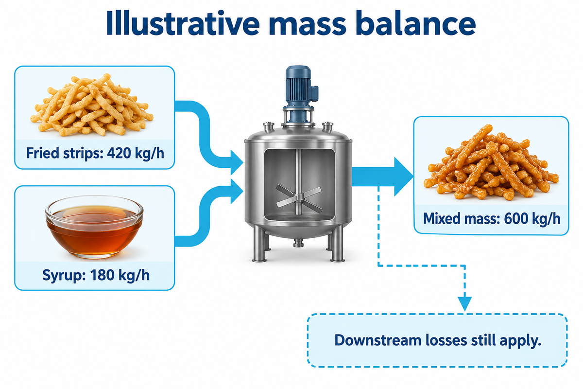
Assume a recipe contains 70% fried strips and 30% syrup by mass at the mixing discharge. Supplying 420 kg/h of fried strips then supports 420 ÷ 0.70 = 600 kg/h of mixed mass, provided 180 kg/h of syrup is available. Cutting and packing losses are still downstream. The assumed recipe fractions aren’t a standard sachima formulation.
Write the measurement point next to every input, before or after draining, before or after addition of syrup, or before or after rejection. Material requirements planning should use the recipe mass balance; purchasing a higher-rated fryer cannot replace missing syrup or packaging material.
Disclosure of one process, CN105472988A, describes fried dough with syrup and subsequent cooling/forming. Listed assignees are companies related to Nestlé. It is useful process context, not a UDTECH patent or a recipe specification for this calculation.
Mass-basis check. In the assumed 70:30 mixture, 420 kg/h of fried strips and 180 kg/h of syrup meet at 600 kg/h before downstream losses. Ask a supplier to name the weighing point before comparing that figure with a 1,000 kg/h finished-mass rating.
Calculate saleable shift output with one loss model
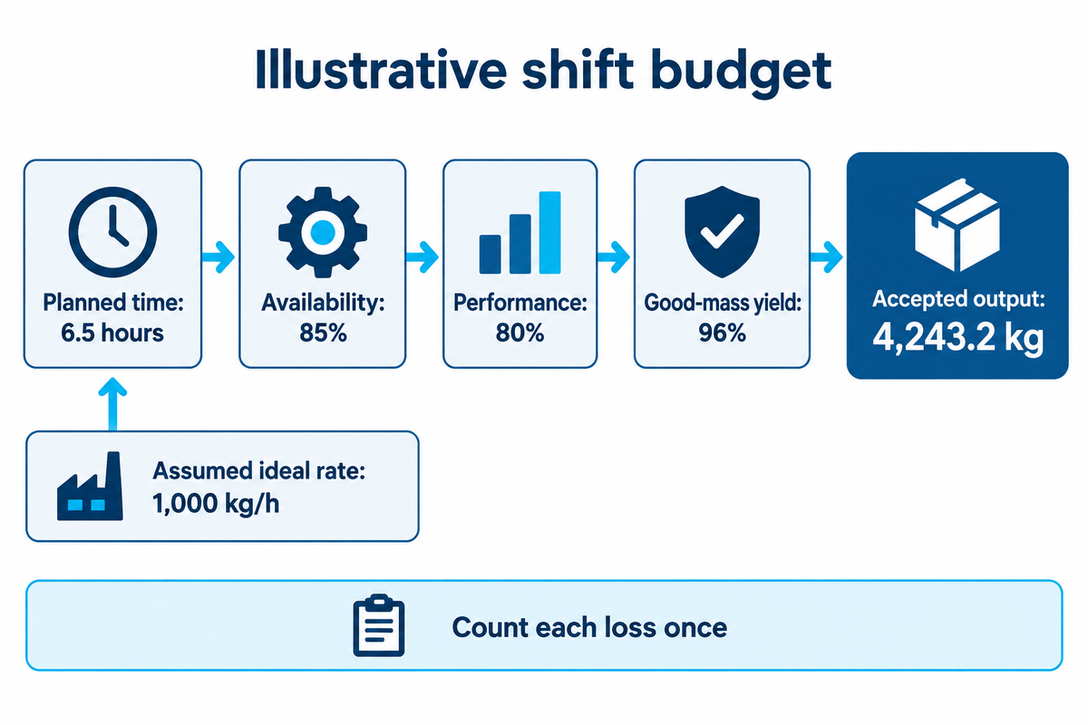
Estimate saleable shift output by multiplying an ideal rate by planned production time and distinct availability, running speed and quality factors. Use each factor only once. In the case of actual output being assessed as good kg/planned hour, multiply that rate by the same planned hours without any loss deduction.
The Vorne calculation method defines availability against planned production time, performance against an ideal running rate and quality as good output divided by total output. Rates and quantities must refer to one recipe and measurement boundary.
Demand-to-Dispatch Capacity Budget
Consider an illustrative 480-minute shift. Exclude 90 minutes when production isn’t scheduled, leaving 390 minutes, or 6.5 hours. Assume an independently established ideal rate of 1,000 kg/h, availability of 85%, performance of 80% and good-mass yield of 96%. The ideal rate here’s a scenario assumption, not automatically the brochure rating.
| Step | Calculation or input | Result | Meaning |
|---|---|---|---|
| 1. Scheduled shift | 8 × 60 minutes | 480 min | Calendar window |
| 2. Excluded time | Declared nonproduction | 90 min | Outside planned production |
| 3. Planned production | 480 − 90 | 390 min | 6.5 planned hours |
| 4. Ideal rate | Assumed recipe-specific rate | 1,000 kg/h | Same final-mass basis |
| 5. Availability | Run time ÷ planned time | 85% | 5.525 running hours |
| 6. Running performance | Actual ÷ ideal running rate | 80% | 800 kg per running hour |
| 7. Gross shift output | 5.525 × 800 | 4,420 kg | Before rejects |
| 8. Good-mass yield | Good mass ÷ gross mass | 96% | Rejects counted here |
| 9. Accepted shift output | 4,420 × 0.96 | 4,243.2 kg | At the agreed boundary |
| 10. Planned-hour good rate | 4,243.2 ÷ 6.5 | 652.8 kg/h | All three losses already included |
The complete calculation is 1,000 × 6.5 × 0.85 × 0.80 × 0.96 = 4,243.2 kg . Alternatively, 768 good kg/h × 5.525 running hours yields the same answer. Multiplying the measured 768 kg/h by performance and quality again would result in an understatement.
Common mistake: subtracting a changeover from the calendar and also charging the same minutes to availability. Decide which bucket owns the stop. The Vorne loss-classification FAQ helps distinguish planned stops from time outside the production schedule.
Use good mass yield for a kilogram budget. A good-piece count ratio gives the same mass relationship only when piece weights are equivalent. Reconcile weigh records if rejects are systematically heavier or lighter than accepted bars.
One-rate rule. An assumed ideal 1,000 kg/h becomes 652.8 accepted kg per planned hour after the stated factors. A measured 652.8 kg/h on that same basis already contains those losses. Applying them again would create an artificial capacity gap and could trigger an unnecessary purchase.
Find the bottleneck across batch and continuous stages
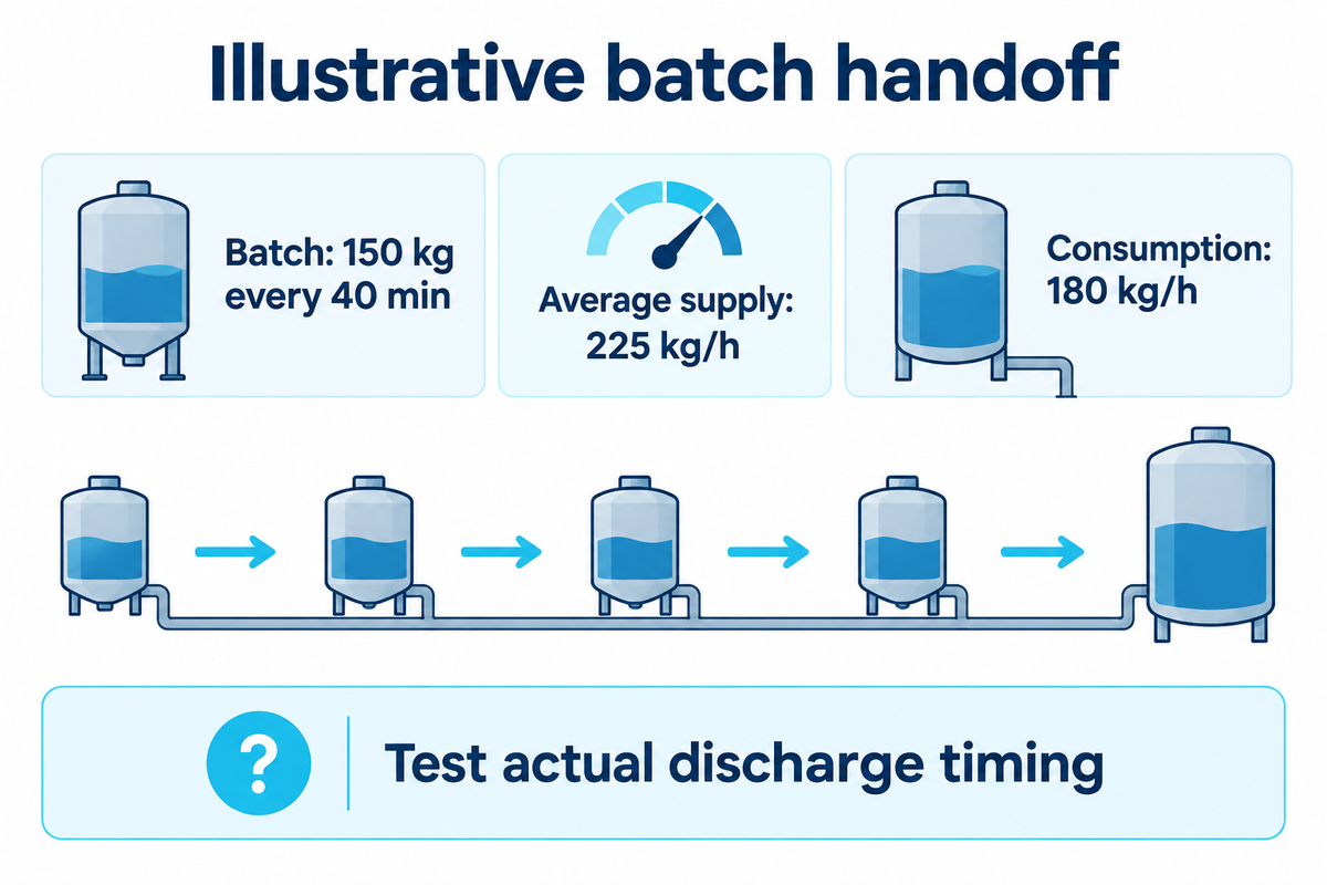
Compare complete batch cycles with continuous consumption. Check the actual delivery sequence between stations. A kettle can provide enough syrup per hour on average yet leave the mixer waiting between discharges. Sustainable manufacturing capacity depends on the entire manufacturing process (the complete process of refilling, heating, discharging and cleaning).
Assume one kettle supplies 150 kg per complete 40-minute cycle. Average syrup supply is 150 × 60 ÷ 40 = 225 kg/h. At the assumed 30% syrup fraction, that’s equivalent to 750 kg/h of mixed product before downstream losses. A 600 kg/h mixing target needs 180 kg/h of syrup, so average supply has headroom.
Headroom isn’t a delivery schedule. Inventory management must also track when each usable batch arrives. Draw each batch’s ready time, discharge interval and usable holding quantity against mixer consumption. A 150 kg charge covers 50 minutes at 180 kg/h; this doesn’t establish that the vessel can refill while discharging or that syrup may be held for 50 minutes. Site recipe and quality controls dictate holding conditions.
To perform a discrete event check, start with the actual initial buffer, then add all usable discharges and subtract consumption for each interval. Stop when the inventory goes to zero, exceeds usable storage or breaches a recipe limit. NIST’s research on finite-buffer scheduling examines the relationship of buffer size and operating policy. Its model doesn’t produce a universal sachima factor.
Batch handoff. A hypothetical 150 kg syrup batch every 40 minutes averages 225 kg/h. Against 180 kg/h consumption, the arithmetic shows 45 kg/h of average headroom. The acceptance question is whether the actual discharge sequence keeps the mixer supplied within the limits of storage and holding.
Size cooling and buffers from residence time
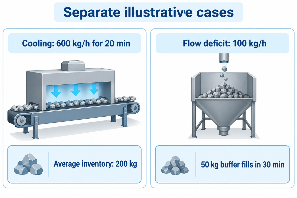
Average inventory is determined by product flow and validated residence requirement, and usable storage is tested against interruptions. Cooling inventory is product held up in a normal part of a process; a buffer absorbs a transient difference in processing times. Neither calculation establishes belt dimensions or a safe holding period without product trials and an agreed loading arrangement.
MIT’s explanation of Little’s Law relates average inventory, flow and time in a stable system. For a 600 kg/h stream requiring on average 20 minutes to cool, average inventory is 600 × 20 ÷ 60 = 200 kg. Other design inputs include density, bed depth, belt coverage, and airflow.
Now consider a separate mismatch: an upstream stage supplies 600 kg/h while downstream can take only 500 kg/h. With 50 kg of free storage, the queue fills in 50 ÷ 100 = 0.5 hours, or 30 minutes. Adding storage delays the stop; it does not remove the persistent 100 kg/h deficit.
If the conveyor is proposed to be longer, what problem is the proposal solving? More residence inventory could be required by the recipe which is supported by the validation, while temporary accumulation requires free space and a restart strategy. Include startup and shutdown events; a steady-state average does not show either transient.
Cooling boundary. At an assumed 600 kg/h, 20 minutes corresponds to 200 kg of average inventory. A 100 kg/h deficit downstream fills 50 kg of buffer in 30 minutes. Specify the processing residence requirement and the free accumulation capacity separately.
Match wrapper capacity to the smallest bar
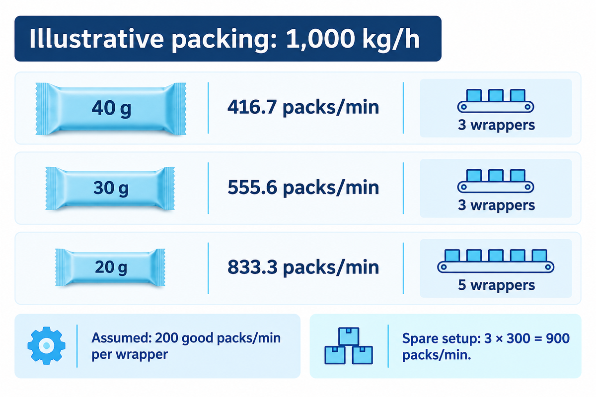
Mass flow of wrapper-ready product in bars must be converted to accepted individual packs per minute using actual mean bar weight. Then divide by the sustainable good-pack rate of each wrapper over the same time window and round up. Smaller bars raise piece demand, while existing idle capacity can prevent an increase in installed machine count.
For one bar per pack, packs/min = kg/h × 1,000 ÷ bar grams ÷ 60. Use actual mean accepted grams rather than blindly substituting the label. Overfill consumes mass, and rejection based on weight can reduce the saleable count. NIST distinguishes average contents from individual package variation. The calculation for capacity requires both weighing and reject records.
Gram-to-Wrapper Switchpoint Chart
| Actual mean bar mass | Required good packs/min | Assumed good rate per wrapper | Minimum wrappers |
|---|---|---|---|
| 40 g | 416.7 | 200 packs/min | 3 |
| 30 g | 555.6 | 200 packs/min | 3 |
| 20 g | 833.3 | 200 packs/min | 5 |
All wrapper rates in this chart are assumed sustainable values and not machine specifications. If measured good packs/min already includes stoppages and rejects for the selected time window, don’t apply another blanket efficiency factor. Multi-bar packs require a different piece to pack conversion.
Suppose a factory already has three wrappers, each sustaining 300 good packs/min on the same basis. Their combined 900 packs/min covers both the 30 g and 20 g scenarios. With the 50% increase in pack work, the minimum installed count still remains at three. Product feeding, film changes and downstream case packing must also sustain this increased work.
The named specialists in Baking & Snack’s conveyor and packaging report describe the need to reconcile mass flow with pack sizes. Apply that principle to bar, film and feeding arrangements that you’ve tested rather than depend on the bagger’s catalog speed that you’ve borrowed.
Switchpoint for wrapper at 1,000 kg/h. At 1,000 kg/h, a 20 g bar needs about 833.3 packs/min against 555.6 for a 30 g bar. Five assumed 200-pack/min wrappers cover the smaller bar, with three assumed 300-pack/min wrappers covering it as well. Spare capacity changes the investment decision.
Stress-test the production schedule before adding a shift
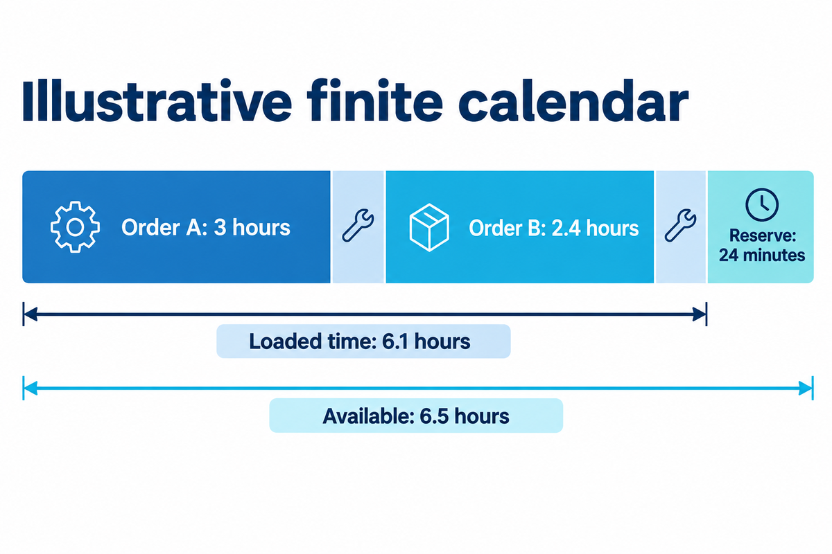
Load net good-production hours and sequence-dependent changeover time for each product into the available calendar. Reserve shared operators and syrup preparation and packing resources in the same calendar. Finite capacity planning makes a master production schedule feasible only when every required resource is available at the time the job needs it.
In an illustrative shift, order A needs 1,800 kg at 600 accepted kg/h, or 3 hours. Order B needs 1,200 kg at 500 accepted kg/h, or 2.4 hours. Two changes taking 0.35 hours each bring total loading to 6.1 hours. Against 6.5 available hours, the reserve is 0.4 hours, or 24 minutes. These net good rates already take into account expected production losses.
Changeover time may be dependent on direction. Different inclusions or allergen profiles can require a particular sequence and cleaning process. Use your site’s established controls and measured durations. The FDA’s process discussion mentions that scheduling and cleaning are pertinent controls; it provides no standard changeover time for this case.
“Running at 100% capacity is very difficult on resources”
That dated observation of the bakery supports leaving a reasoned reserve, not imposing a universal utilization target. An overloaded packing crew can remain the constraint even after processing machine hours double. Check labor availability, maintenance coverage and material replenishment, before approving a second shift.
Calendar test. The assumed 3,000 kg mixed order occupies 6.1 hours after two 21-minute changes. A 6.5-hour window leaves 24 minutes. Any extra cleaning, waiting or shared-resource conflict larger than that reserve changes the dispatch decision; a second shift needs its own resource calendar.
Choose the capacity change that removes the constraint
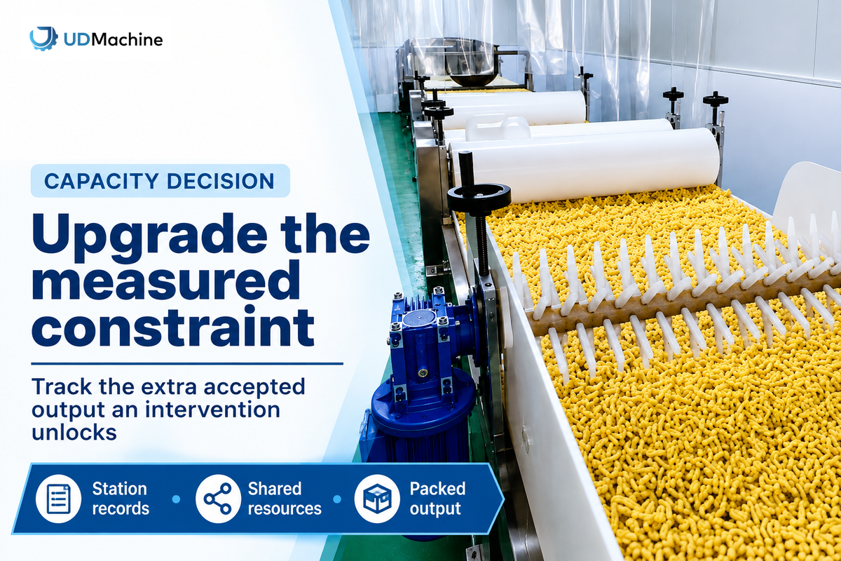
To optimize usable capacity, pick an intervention from the measured constraint and the output it prevents you from dispatching. Increased frying capacity helps only when downstream stages can accept increased flow. Recovering an idle nonconstraint may improve a local utilization number without increasing good packed output or shortening order lead time.
An adjacent FANUC case at Brunos describes manual downstream packing lagging automated food processing. It illustrates the handoff problem; its equipment and results aren’t sachima performance benchmarks. Use station records to identify your own capacity gaps.
| Observed pattern | Likely capacity class | Record to check | First decision |
|---|---|---|---|
| Mixed mass short of target | Mass-basis mismatch | Recipe and weighing points | Normalize station rates |
| Mixer waits between batches | Batch timing | Ready and discharge times | Test delivery sequence |
| Cooling queue keeps growing | Sustained downstream deficit | Arrival and exit kg/h | Balance flow rates |
| Queue appears only during film changes | Temporary interruption | Stop duration and free buffer | Check accumulation and restart |
| Small bars overload wrappers | Piece-count constraint | Actual grams and good packs/min | Calculate required count |
| Wrapped bars await cases | End-of-line labor | Case-pack and pallet pace | Include dispatch boundary |
| Second shift misses targets | Shared-resource conflict | Staff and kettle calendar | Resolve resource allocation |
| Rated speed exceeds good rate | Loss or rating-basis gap | Runtime and rejects | Reconcile the rate path |
| Output depends on SKU order | Sequence-dependent setup | Routings and cleaning records | Resequence within site controls |
| Plant can produce but cannot dispatch | Supply-chain restriction | Film, cases and shipping windows | Reconcile demand and supply |
Compare interventions for additional accepted kilograms within the allotted time frame and the resources consumed. Capacity utilization is good evidence, but strategic planning shouldn’t reward running every machine to improve its percentage. For process faults other than sizing arithmetic, consult the sachima troubleshooting and acceptance guide.
Turn the capacity budget into a supplier handoff
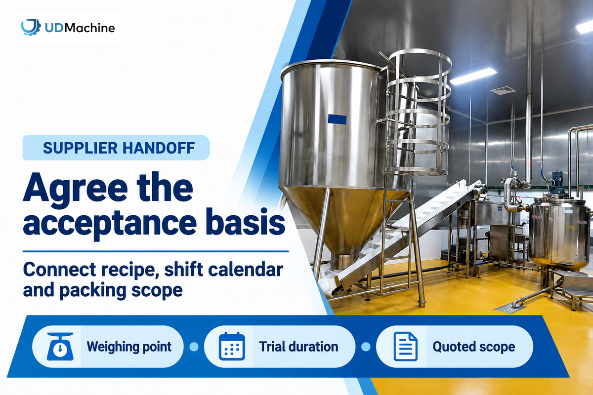
Provide an acceptance basis that integrates the recipe, output boundary, shift calendar and packaging requirement with the supplier. Request a representative combined-line demonstration against that basis. Manufacturing capacity becomes commercially useful when the two sides agree on what’s weighed, what losses are included and what downstream operations are included in the quoted scope.
The YT-30 sachima line and quoted station scope publishes a rated 1,000 kg/h. Its listed eight-station core ends at shaping and cutting; packaging is separate unless included in the quotation. UDTECH’s company and manufacturing background helps identify the supplier, while a recipe-specific trial establishes the relevant operating evidence.
Send the accepted kilograms daily by SKU, the actual piece weights, the planned pack format, complete batch cycles, and the shift calendar. Also, send the cooling requirements from your process team, all shared resource limits and the starting and ending condition of the inventory. Also, ask for the duration of the trial and the startup treatment, rather than just a brief peak reading.
The existing timed sachima output record can turn a weighed test sample into a measured good-product rate. Extend that record across representative recipes, interruptions and shifts before using it for recurring customer commitments.
ISO 22400-2’s public scope supplies context for consistent formula elements, time behaviour and units. As checked in October 2026, the catalog lists the 2014 publication and its 2017 amendment, with a revision in development. This reference does not certify the equipment.
Plan for smaller packs without inventing a demand forecast
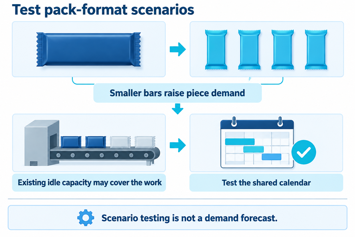
Instead of relying on an assumed sachima growth rate, take advantage of changing pack formats as scenarios in capacity management. A smaller bar can increase packaging work before it changes processing kilograms. Test that workload against sustainable wrapper output, feeding behaviour and film-change occupancy before selecting food machinery or committing to a new promotion.
PMMI’s January 2025 snack-market report for instance mentions shifting pack-format variety and machinery investments. Its snack-industry survey is context for scenario testing, not a sachima-specific demand forecasting series.
Set a planning cadence. Update the next dispatch schedule when orders change. Review the product family mix with commercial staff. Re-evaluate strategic network planning when the planning horizon or the facility allocation changes. A simple planning tool with dated inputs can identify capacity requirements before a large planning system becomes justifiable. Rough cut capacity planning screens aggregate loading; finite scheduling resolves the actual shared calendar.
A plant evaluating formal optimization can later use mixed integer programming to allocate jobs and setups. Such a model requires reliable routings and batch data. For the current decision, make capacity assumptions visible, resolve the measured constraint and keep the capacity planning process tied to saleable output.
Start creating your sachima shift budget with UDTECH. Send daily kilograms, SKU weights, shift hours available and packing format. Use the sachima production line scope as the starting point for a matched processing and packing discussion.
Frequently Asked Questions
Are planned maintenance, holidays, and changeovers included?
Maintenance, holidays and changeovers belong in the capacity budget once, within the agreed calendar and loss definitions.
Include every occupied period once, using the calendar and loss definitions agreed for the budget. Holidays and full shutdowns normally reduce the available calendar before jobs are loaded. Within a scheduled production window, maintenance or changeovers must appear either as explicit reserved time or in the measured availability basis. Subtracting the same stop through both routes understates capacity and can make an otherwise feasible schedule appear overloaded.
What data do planners need for accurate capacity planning?
Accurate planning needs dated demand, mass-balance, time, output and shared-resource records for each SKU.
Collect accepted demand by SKU, recipe mass balance, actual bar weights, scheduled and running time, sustained good output and reject records. Add complete batch cycles, validated cooling requirements, usable buffer capacity and measured wrapper performance. A dated shared-resource calendar is also necessary: operators, syrup preparation and case packing may constrain the plan. Mark assumptions separately from measured inputs, then replace the uncertain values through representative trials.
What is the difference between finite and infinite capacity planning?
Finite planning fits jobs into actual resource limits; infinite planning loads requested work without proving that fit.
Infinite planning loads requested work without proving that machines and shared resources have enough available hours. Finite planning places jobs within the actual capacity limits and setup sequence. For a sachima plant, including only the fryer is insufficient: syrup supply, cooling, wrappers and labor must also fit. Rough-cut capacity planning is an early aggregate screen; the detailed schedule needs the resource and timing constraints.
Can a larger fryer increase dispatched sachima output?
A larger fryer adds dispatched output when it is the measured constraint and downstream stages can accept the extra flow.
Yes, when the fryer is the measured constraint and syrup supply, cooling, wrapping and dispatch operations can sustain its extra finished-mass-equivalent flow. Otherwise, the upgrade may mainly increase waiting inventory.
Can one factory trial settle every SKU’s shift capacity?
A factory trial establishes capacity evidence for the conditions actually tested.
One trial establishes evidence for its tested conditions. A broader production commitment needs records covering the recipes, bar sizes and operating windows that will actually be sold. Keep the measurement point, actual mean grams, reject rule and startup treatment with the result. A 30 g bar trial can’t by itself settle the packing requirement for a 20 g bar, because the same mass flow requires more pieces per minute.
Extend the test plan to representative batch delivery, cooling occupancy and the site’s required changeover sequence. Run the shared-resource calendar as well: a second shift may have different staffing or preparation support. Finally, reconcile starting and ending work in process so an apparent output increase doesn’t merely consume stored upstream product. Agree the acceptable test duration and repeat conditions with the supplier before turning a short sample into a recurring shift target.
References & Sources
- Vorne: OEE calculation definitions and loss-classification FAQ.
- MIT: Little’s Law and queueing tutorial.
- NIST: scheduling with dedicated finite buffers.
- NIST: average and individual package contents.
- Baking & Snack, 2020: conveyor and packaging capacity.
- Baking & Snack, 2016: Todd Wallin interview.
- FDA: process sequencing and cleaning discussion; historical labeling passages are outside this article’s scope.
- FANUC: Brunos downstream packaging case.
- ISO 22400-2 public catalog; publication status checked October 2026.
- PMMI, January 2025: snack-market format and investment context.
- CN105472988A: original process disclosure and listed assignees.